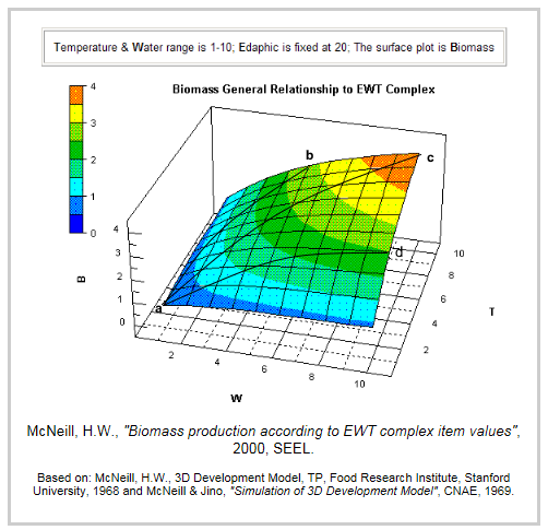
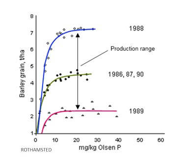
All of the factors additional to fertilizer that affect yield have states determined by the location of the experimental plots. Thus the weather factors of temperature and rainfall that were predominant in the different years and the natural fertility of the soil are all specifically related to the geographic location of the experimental plots (space dimension) and the conditions in the year concerned (time dimension). The reason soil texture (particle size) is important is because this determines the water holding capacity of a soil. Large particles, sandy soils, allow water to drain away. Silts with intermediate sized particles, have a better water holding ability and the water remains accessible to plant roots. Clays hold water tightly due to capillary effects meaning that in drier periods the tension is too high for plant roots to extract water. Water availability to crop roots is measured as water deficit which is the difference between rainfall and evapotranspiration and the water holding capacity of the soil (texture effect). Just to complete this explanation, ambient temperatures vary with the altitude of a site losing 0.6^oC to every 100 metres gain in altitude. Ambient temperatures difference of just 3^oC can have an impact on the average rate of photosynthesis leading to up to a gain in yields of around 20%-25%. This locational-state space dimension can be used to interpolate temperatures and expected yields according to their altitudes against a reference site with a known temperature, altitude and yield. The conclusion of this introductory section to locational-state is that quite often, to simplify statistical analysis and important determinant mechanisms or relationships are ignored. On the other hand, the contributions of these factors to the result are often not quantitatively measured.

Main take-away: Such correlative statistical analysis informs us of a basic relationship but this provides only a rough guidance for a farmer to understand the financial results of any production year and what might be done to make use of this information, according to a farm's location, in order to optimize production inputs.

How does this relate to monetarism?

In the case of economic activities, most systems have a similar physical production response curve to physical inputs as illustrated in the case of biomass production. Human learning and the rise in operational competence also follows a similar growth curve (learning curve). Therefore it was realized there is a similar "production function" that unified the biomass production surface with economic processes from manufacturing to heavy industry and to services and including human learning. This the reason locational-state analysis progressed to become a Locational-State Theory because it has a universal application.

However, just as in the case of the farming scenarios, any economic policies where policy instruments have the purpose of influencing events so as to achieve a policy target, it is necessary to identify the mechanisms whereby this cause and effect is supposed to take place. In the case of the staple logic of monetary instrument impacts, the Quantity Theory of Money (QTM) has been shown to lack critical variables for it to have any utility in calculating outcomes (see, "Why monetarism does not work" or, "A Real Money Theory").

Besides the flawed nature of the QTM, monetarists ignore the processes whereby economic growth occurs without inflation. Here we refer to the role of change or innovation in technologies and technique that can raise productivity, lower unit costs, raise margins and enable rises in real incomes through price moderation or even reductions (see, Technology, technique and real incomes). However, these mechanisms, which almost never feature in any monetarist policy logic but they are the determinants of inflation.

Lastly, the assumption that inflation is caused by excessive demand and is controlled by reducing disposable funds for consumption has no mechanism associated with this logic. As in the case of agricultural experimental results and theories built upon these, a considerable amount of information on the locational-state dimensions are missing from monetary policy logic with any models being virtually non-existent.

Economic growth

Growth takes place as a result of changes in consumption levels and in levels of production and associated productivity. Unit prices are set in a dynamic process of "price discovery" where final prices are arrived at as a trade-off between the producer securing what is considered to be a reasonable compensation and the consumer purchasing their needs within the existing range of their available disposable incomes. Therefore the levels of economic activity are determined by what is happening to productivity and disposable incomes. In the end most disposable incomes, or wages, are paid through employment in goods and services production activities.

During periods when existing or new advanced in technologies and techniques provide opportunities for companies in all sectors invest to improve performance relevant to their specific types of activity, investment activities occur.

Growth and absorptive capacity

However, there is a specific limit on rates of productivity growth associated with the adoption of new technologies and techniques governed by the delays involved in investments having an impact on productivity. These delays are very often linked to the workforce learning how to adapt to the new technologies and other organizational adjustments. As a result rational investments seldom have an immediate impact on productivity. Delays between a new system being commissioned as being in working order to the time where target productivity levels are achieved can vary from between a short time to in excess of 10 years.

The geographic diffusion of innovation The case of more productive hybrid corn in the USA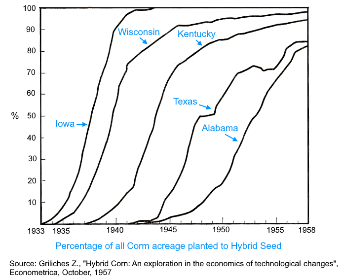 All innovations have an associated locational-state time and space components which impact the effectiveness of policy within electoral cycle time frames.

This is because, for example, introducing a systems component to increase throughput requires the eventual expansion in the handling capacity of all downstream processes, including logistics. Therefore there is a location-state time-based component which will determine the timing of an investment and the attainment of a desired impact. As a result of these common facts there is a specific limit on the absorptive capacity of the economy for finance for such investment. If money volumes applied to productive investment falls within these bounds there is no reason why there should be any inflation. This point was made by Nicholas Kaldor when countering monetarist reasoning concerning inflation.

Where money volumes exceed the absorptive capacity of the productive supply sector's investment needs, the funds tend to flow into assets including, land and real estate, offshore investment, financial instruments, shares, rare objects, crypto-currencies and precious metals as well as non-productive credit for purchases of consumer goods and services. As explained below, it is these monetary flows which build up an inflationary bubble.

Where a manufacturer of a product which can augment productivity, such as automation equipment, this company itself might not exhibit increases in productivity other than increases in sales. The same company might also not register high profits because it is reinvesting in its own production using own funds. The impacts of the sales to other companies are what will impact the productivity of companies in various locations. Therefore there is a locational-state geographic-based component as to where productivity increases will take place subject to the learning issues mentioned before (see right).

Competition

In reading the following sections it is as well to keep in mind the significance of price discovery in maintaining the opportunity for companies to maintain competitive prices. Simple because more money flows into the economy does not mean companies somehow lose sight of the fact that they maintain their market share by maintaining a competitive price-setting activity. Similarly in time of depression some companies will attempt to maintain or even increase their market share by making marginal reductions in their unit prices.

In a competitive economy, the only reason a company will voluntarily raise output prices is because they are forced to as a result of rising costs and not as a result of "demand".

Note that rising costs are the inputs and determinants of the mechanism of corporate price-setting that leads to rising unit output prices, inflation has nothing to do with "demand". Prices can rise temporarily when there is short supply and consumers are prepared to pay more to secure their needs..

Therefore it is important to keep these facts in mind when reviewing inflationary and deflationary market conditions.

Inflationary scenario

Where there is a low interest rate and the central bank is encouraging an increase in money volumes the flow of funds would normally go into productive investment as well as assets. Asset prices such as land, housing, office space, wholesale warehouses and industrial units tend to rise and this inflation leaks into the costs of the productive sector. This is because asset holders wish to receive a level of return that is proportional to the asset value. Because of rising costs companies might raise loans to invest in technologies to compensate for these cost rises by raising their productivity. However, as explained, the realization of cost savings will take time as a company adjusts to the new system, the workforce comes up to speed and refines its handling of the process. The ability to avoid increasing unit output prices can become difficult because of the additional costs of the repayment of the loan. Therefore some companies will raise their prices. Although the central bank inflation target of 2% per annum appears to be low it is equivalent to a decrease in purchasing power of around 18% each decade. However, when this level is reached a central bank would normally raise base interest rates which would reduce the feasibility of some investment plans and raise premiums on existing loans causing more pressure on costs. In the meantime, the rise in interest rates also impacts consumer spending resulting in a fall in consumption purchases on credit. The government might raise income tax slightly resulting in consumption falling further. The knock-on effect is that companies end up with over-capacity leading to a rise in overhead costs/unit of output and higher unit costs of operation.

At the macroeconomic level changes in productivity arising from the diffusion of innovation occurs as a result of multi-layered diffusion cycles each with a different duration and geographic spread to the point of attainment of productivity objectives. 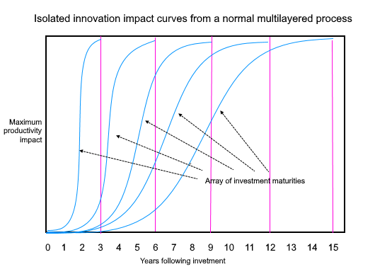Most governments and central banks are not in possession of the requisite level of detail on the diffusion of productivity-enhancing innovations and therefore do not have the data upon which to base policy decisions on the impact of interest rates and monetary volumes on the real economy performance. Therefore, they have no basis to guide policies aiming to achieve real incomes growth.

Under such circumstances it is difficult to pay higher wages and gains in real incomes arising from lower unit prices become difficult to realize and there might be labour lay offs.

Therefore the relationship of productivity, growth and unit prices to interest rates could have almost no discernible relationship because of the locational-state time and geographic based nature of the diffusion of productivity through the economy.

Governments might assume that rises in productivity during a high interest rate period vindicates the policy action in "getting rid" of inflation when in fact the productivity investment had been made before any change in interest rates.

Deflationary scenario

When inflation remains well below 2% per annum central banks take this to be a situation where there needs to be "more demand" fed into the economy. However, low inflation is usually the result of the benefits of the deflationary impact of investments in technological advance and raised productivity which absorbs inflation while enabling the prices of some products to fall. This has the effect of raising the purchasing power of wage earners. Therefore, although nominal disposable incomes are static the real income of the population rises with the rise in purchasing power as a function of unit prices declines.

Under such circumstances the interpretation of this as being a decrease in demand reflects misunderstanding of the difference between nominal and real growth and as a result, heralds a fall is interest rates and the promotion of rises in money volumes. As previously stated the productive supply side has a limited absorptive capacity for productive investment, so with low interest rates there is a considerable rise in the volume of funds flowing into asset markets causing speculative price inflation, which eventually leaks through into to production costs This initiates a new inflationary cycle

Besides land and real estate price inflation the low interest rate high money volume policy, such as quantitative easing, results increased flows into offshore investment, lowering the future employment base onshore, as well as share buy backs which increase share prices and destroy meaningful price-earning ratio levels. Other "investments" include financial instruments such as derivatives and options and including crypto currencies and rare objects and art. With such low interest rates the ability to drive up speculative prices in asset markets becomes more attractive that what appear to be higher risk productive supply sector investments. Indeed, the supply side productive sector faces rising interest rates from banks whose preference is to support speculative asset purchases for large clients as well as on their own account to satisfy shareholders. As a result, in spite of the fact base interest rates are low, banks raise their interest rates to supply side productive companies causing this sector to be without easily accessible finance resulting in difficulty in raising finance on reasonable grounds for investment.

Incomplete and complete data sets

Because of the very variable time bases and geographic diffusion of the impacts of investment in more productive technologies it is virtually impossible to use any of the annual data series on inflation, economic growth (consumption or "demand") and unit prices to draw any conclusions of the effectiveness of policy instruments in controlling inflation because of the range of lags concerned. Compared with electoral cycles of at a maximum of 5 years it is therefore virtually impossible to correlate any changes in productivity, inflation control or turnover within any administration resulting from monetary policy or fiscal decisions taken by the government concerned. As a result, the consequences of monetary econometrics based on incomplete datasets, lacking the locational-state detail, is more than likely to draw inconclusive or even inverse to expected conclusions. Since this data does not exist in a readily accessible form because it is not collected in a coherent and organized fashion, one has to ask what is the worth of monetary theory and derived policies from the standpoint of the majority constituents of this country? What are the criteria for monetary policy decisions?

As Luwig von Mises observed, there is a serious calculation and knowledge problem on the part of governments and central banks when they attempt to apply such centralized policies. In the discussion above it is evident that there is a lack of coherent theory and practice associated with monetary policies. There is only a revealed preference towards the maintenance of asset "values" in upswings and down swings creating a collateral damage measured in terms of employment levels, declining wage levels, rising unit prices and therefore falling real incomes. It is more than evident that such a limited focus on assets, openly admitted by central banks to be the "stabilizing factor", is assumed to result in investment and "trickle down" benefits for the "masses", is a dishonest proposition because there is no evidence (data) to support this assertion.

Questions that monetarists need to answer

Without access to quite detailed locational-state data, it is difficult to obtain a data set that has sufficient detail to construct a model of any of the mechanisms that link the monetary policy instruments of interest rates and money volumes to inflation control. But monetarists insist that these policy instruments achieve their objectives. Therefore, it would be beneficial if the government and the Bank of England could prepare a document, in plain English, to explain the mechanisms through which they imagine the policy instruments impact inflation to the benefit of the real incomes of wage-earners.

---

¹  Hector McNeill is director of SEEL-Systems Engineering Economics Lab

---

All content on this site is subject to Copyright
All copyright is held by © Hector Wetherell McNeill (1975-2021) unless otherwise indicated